What is the Physical Meaning of the Levi-Civita Connection?
A Riemannian manifold is a differentiable manifold endowed with a Riemannian metric. Given a Riemannian metric, the lengths of curves can be defined via integration, and the angle of intersection of two curves is also well defined. However, there is a priori no direct way of aligning neighbouring tangent planes, hence no direct way of measuring acceleration, for example.
A connection defines the rate-of-change of a vector field. There are many possible connections, hence it is natural to ask what connection to use, and whether on a Riemannian metric there is a canonical choice of a connection. The answer to the first question is, of course, that it depends on what you are wanting to do. (On a Lie group there are several interesting connections, for example.) This short note focuses on the second question.
The canonical choice of a connection on a Riemannian manifold is the Levi-Civita connection. Why is it a natural choice though, and what is its physical meaning?
The short answer is that it corresponds to the parallel transport which would naturally occur if we were living on this manifold. For example, if we are told to walk in a straight line with zero acceleration, we could do this on our planet without defining a connection. How? We simply place one foot in front of the other to take our first step, then repeat, each time doing our best to walk in a straight line. What actually happens is gravity pulls our foot back to Earth and hence we end up walking in a great circle.
Similarly, if we walk while holding a lance, and are told not to move the lance as we walk, we are actually defining a rule for parallel transport.
Put simply, the Levi-Civita connection corresponds to the rule for parallel transport that results by walking along the curve without moving the vector/lance. Gravity will cause additional movement to ensure we stay on the surface of the planet and this is what is captured by the Levi-Civita connection.
Technically, it is not gravity but merely projection back onto the surface of the manifold. Specifically, by the Nash embedding theorem, any Riemannian manifold can be isometrically embedded into Euclidean space. Then walking “in a straight line” on the manifold is achieved by taking a step in Euclidean space then projecting back down to the manifold (just as gravity would pull your foot back to the ground). Then take the limit as the step size goes to zero.
For additional details, see my response here: https://mathoverflow.net/questions/376486/what-is-the-levi-civita-connection-trying-to-describe/376593#376593
The Twin Capacitor Paradox
With COVID-19 causing a transition to online teaching, I am now in the habit of making short videos…
Consider two isolated capacitors, one with a charge on it, one without. Then suddenly bring them together. The charge will distribute equally on the two capacitors. But energy will have been lost! Where did it go?
A Note on Duality in Convex Optimisation
This note elaborates on the “perturbation interpretation” of duality in convex optimisation. Caveat lector: regularity conditions are ignored.
Recall that in convex analysis, a convex set is fully determined by its supporting hyperplanes. Therefore, any result about convex sets should be re-writable in terms of supporting hyperplanes. This is the basis of duality. A simple yet striking example is Fenchel duality which is nicely illustrated in the Wikipedia. Although it relies on the Legendre transform, which I have written about here, the current note is self-contained: it explains the Legendre transform from first principles.
Let’s start with a classic example of duality. In its usual presentation, it is not at all clear that it relates to the aforementioned duality between convex sets and their hyperplanes. Nevertheless, before presenting a general method for taking the dual of a problem, it is useful to have a concrete example at hand.
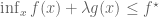
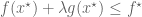
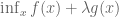
Consider minimising 


Remark 1.1: One way to “understand” this duality is by understanding when it is permissible to replace 


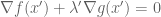
Remark 1.2: The dual appears to relate to the method of Lagrange multipliers. (See here for the physical significance of the Lagrange multiplier.) This makes sense because there are only two cases. Either the global minimum of 

Remark 1.3: If the global minimum of 


Remark 1.4: If the global minimum of 


Remark 1.5: A benefit of the dual problem is that it has replaced the “complicated” constraint 
While we have linked the dual problem with Lagrange multipliers to explain what was going on, it is somewhat messy and requires additional assumptions such as differentiability. Furthermore, the dual problem was written down, rather than derived. The remainder of this note attempts to rectify these issues.
The Legendre Transform and Duality
Let 


We will be lazy and write “supporting hyperplane of
A hyperplane is of the form 


It is straightforward to derive a formula for 
For 

We therefore define 
The original claim is that 

It is striking that this formula has exactly the same form as the Legendre transform! Indeed, the Legendre transform is self-dual: the above can be rewritten as 
At this juncture, it is easy to state the algebra behind taking the dual of an optimisation problem. In my opinion though, there is more to be understood than just the following algebra. The remainder of this note therefore elaborates on the following.
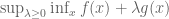
Given a convex function 


For reasons that will be explained later, the “trick” is to define 


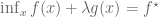
By definition, 

Duality: 
While the above algebra is straightforward, a number of questions remain.
- What is going on geometrically?
- Why should the left-hand side be easier to evaluate than the right-hand side?
- How should the family
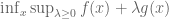
It is remarked that if we are allowed to interchange 


A Geometrical Explanation
The aim is to understand geometrically what the left-hand side of the equation labelled Duality is computing. Start with the term 


For a given 


The first key observation is that because the hyperplane 

To prove the assertion that 


We are halfway there. Given an orientation 

To help focus on the implicit function 


Geometrically, recall that 


Algebraically, start by recalling from earlier that we have shown a property of the Legendre transform is that 


What we have shown is that if 


Summary: To find 


Remark: While introducing points
An Example of When the Dual Problem is Simpler
The Duality equation is only useful if solving 
Consider the constrained optimisation problem introduced near the start of this note: minimise 

In convex optimisation, a constrained optimisation problem can be written as an unconstrained (but discontinuous and therefore still “difficult”) optimisation problem simply by defining the value of the function to be infinity at points violating the constraint. One way to write this is as 


Consider evaluating 


Finally, it is mentioned that for this example, the left-hand side of the Duality equation becomes
How to Choose an Embedding?
First, a remark. One might ask, why not look for a function 
Since choosing an extension
To aid visualisation, assume we wish to minimise 


Simply replicating 

We cannot arbitrarily choose values for
Taking 


With these thoughts in mind, we are led to consider choosing 

The reader is encouraged to visualise the graph of 

There is an interesting interpretation of duality in this particular case. Consider 
Simple Explanation for Interpretation of Lagrange Multiplier as Shadow Cost
Minimising 
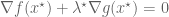


First the reader is reminded why the condition 


To understand the physical significance of 


The key point is to consider what happens if we change the constraint set (the circle) from 


The new value of the objective function, to first order, is given by 

Note that the above is not a proof but rather a rule of thumb that aids in our intuition. An actual proof is straightforward but not so intuitive.
Tennis: Attacking versus Defending
What is an attacking shot? Must an attacking shot be hit hard? What about a defensive shot? This essay will consider both the theory and the practice of attacking and defensive shots. And it will show that if you often lose 6-2 to an opponent then only a small amount of improvement might be enough to tip the scales the other way.
Tennis is a Game of Probabilities
Humans are not perfect. Anyone who has tried aiming for a small target by hitting balls fed from a ball machine will know that hitting identical balls will produce different outcomes. What is often not appreciated though is how sensitive the outcome of a tennis match is to small improvements.
Imagine a match played between two robots, where on average, out of every 20 points played, one robot wins just a single more point than the other robot. This is a very small difference in abilities. Mathematically, this translates to the superior robot having a probability of 55% of winning a point against the inferior robot. (I have used robots as a way of ignoring psychological factors. While the effects of psychological factors are relatively small, at a professional level where differences in abilities are so small to begin with, psychological factors can be crucial to determining the outcome of a match.)
Using the “Probability Calculator” found near the bottom of this page, we find that such a subtle difference in abilities translates into the superior robot winning a 5-set match 95.35% of the time. (The probability of winning a 3-set match is 91%.)
The graphs found on this page show that the set score is “most likely” to be 6-2 or 6-3 to the superior robot, so the next time you lose a match 6-2 or 6-3, believe that with only a small improvement you might be able to tip the scales the other way!
The In-Rally Effect of a Shot
While hitting a winner is a good (and satisfying) thing, no professional tries to hit a winner off every ball. Tennis is a game of probabilities, where subtle differences pay large dividends.
The aim of every ball is to increase the probability of eventually winning the point.
So if your opponent has hit a very good ball and you feel you are in trouble, you might think to yourself that you are down 30-70, giving yourself only 30% chance of winning the rally. Your aim with your return shot is to increase your odds. Even if you cannot immediately go back to 50-50, getting to 40-60 will then put 50-50 within reach on the subsequent shot.
So why not go for winners off every ball? If you can maintain a 55-45 advantage off each ball you hit, you will have a 62.31% chance of winning the game, an 81.5% chance of winning the set, and a 91% chance of winning a 3-set match. On the other hand, against a decent player, hitting a winner off a deep ball is difficult and carries with it a significant chance of failure, i.e., hitting the ball out. Studies have shown that even the very best players cannot control whether a ball narrowly falls in or narrowly falls out, meaning that winners hit very close to the line are rarely intentional but rather come from a shot aimed safely within the court that has drifted closer to the line than intended.
Attacking Options
If by an attacking ball we mean playing a shot that gives us the upper hand in the rally, then our shot needs to make it difficult for our opponent to hit a challenging ball for us. How can this be done?
First, our ability to hit an accurate ball relates to how well we are balanced, how much time we have to react, how fast the incoming ball is, the spin on the ball and the height of the ball at contact. So we can make it difficult for opponents in many different ways. The opponent’s balance can be upset by
- wrong-footing her;
- making her cover a relatively long distance in a short amount of time to reach the ball;
- jamming her by hitting straight at her;
- forcing her to move backwards (so she cannot transfer her weight forwards into the ball).
The opponent’s neurones can be given a harder task by
- giving her less time to calculate how to swing the racquet;
- varying the incoming ball on each shot (different spins, heights, depths, speeds);
- making it harder for her to predict what we will do;
- getting her thinking about other things (such as the score).
Due to our physical structure, making contact with the ball outside of our comfort zone (roughly, between knee to shoulder height) decreases the margin for error because it is harder to “flatten out” the trajectory of the racquet about the contact point.
These observations lead to a variety of strategies for gaining the upper hand, including the following basic ones.
- Take the ball early, on the rise, to take time away from the opponent.
- Hit sharp angles, going near the lines.
- Hit with heavy top-spin to get the ball to bounce above the opponent’s shoulder.
- Hit hard and flat.
- Hit very deep balls close to the baseline.
Each of these strategies carries a risk of hitting out, therefore, it is generally advised not to combine strategies: if you take the ball on the rise, do not also aim close to the lines or hit excessively hard, for example.
If you find yourself losing to someone but not knowing why, it is because subtle differences in the balls you are made to hit can increase the chances of making a mistake, and only very small changes in probability (such as dropping from winning 11 balls out of 20 to only 10 balls out of 20) can hugely affect the outcome of the match (such as dropping from a 91% chance of winning the 3-set match to only a 50% chance of winning). To emphasise, if your opponent takes the ball earlier than normal, you are unlikely to notice the subtle time difference, but over the course of the match, you will feel you are playing worse than normal.
If you are hitting hard but all your balls are coming back, remember that it is relatively easy to return a hard flat ball: the opponent can shorten her backswing yet still hit hard by using your pace, making a safe yet effective return. Hit hard and flat to the open court off a high short ball, but otherwise, try hitting with more top-spin.
Defensive Options
Just as an attacking ball need not be a fast ball, a defensive ball need not be a slow ball. Rather, a defensive ball is one where our aim is to return to an approximately 50-50 chance of winning the point. If we are off balance, or are facing a challenging ball, we cannot go for too much or we risk hitting out and immediately losing the point.
Reducing the risk of hitting out can be achieved in various ways.
- Do not swing as fast or with excessive spin.
- Take the ball later after the bounce, giving it more time to slow down.
- Block the ball back (perhaps taking it on the rise) to a safe region well away from the lines.
- Focus on being balanced, even if it means hitting with less power.
Importantly, everyone is different, and you should learn what your preferred defensive shots are. For example, while flat balls inherently have a lower margin for error, nonetheless some people may find they are more accurate hitting flat than hitting with top-spin simply due to their biomechanical structure and past practice.
Placement of a defensive shot is crucial. Because speed, spin and/or time have been sacrificed for greater safety, it is quite likely that if the opponent has time to get into a comfortable position they can punish your ball. This is yet another example of where small differences can have large consequences: if the opponent can step into the ball you might be in trouble, yet hitting just a metre deeper, or a metre further to the side, might prevent this. Moreover, never forget that placement is relative to where the opponent currently is: hitting deep to the backhand is normally a good shot unless the opponent is already there!
Changes in depth can be very effective but they must be relative to where the opponent is. If an opponent is attacking, she might have moved to being on the baseline, looking to take the next ball early. Hitting a deep top-spin shot, not necessarily very hard, is very effective in this scenario because the opponent is forced to move backwards and thus cannot generate as much power. (A skilled opponent can still hit hard, but even a 10 km/h reduction in ball speed makes a large difference.)
Technical Considerations
Watching the slow-motion clips on YouTube of professional players hitting groundstrokes shows that the same player has many different ways of hitting her forehand and backhand. At the point of contact, you can look to see where her feet are, which way her hips are pointing, which way her shoulders are pointing, the angle of her wrist, and the contact point of the ball relative to the body. And as she hits, you can look to see which parts of the body are moving and which have momentarily become static.
While an upcoming article may consider such technical aspects in greater detail, here it is simply noted that while you should be able to hit every kind of shot from any reasonable contact point, each has advantages and disadvantages. And since tennis is a game of probabilities, it comes as no surprise that the top players instinctively know not just what type of shot to hit but also how technically to hit it in the best possible way for them at that particular moment: if they have time, and want to hit a heavy top-spin, they will probably choose a contact point further away from their body and step into the ball, while if they must return a very fast ball, they may instead use a more open stance and hit the ball more in line with their eyes, well out in front.
Next time you are on the court, experiment with how changing the contact point (even over a relatively small range of 10–20 cm) can change how hard you can hit the ball, how accurately you can hit the ball, and how much top-spin you can generate. And do not forget, this may change depending on the type of incoming ball. For example, generating pace off a slow ball is better done using a different technique than returning a fast incoming ball. Failing to recognise this may mean you “feel” you are not hitting the ball well when in fact you are just not using the best technique for the particular type of shot you want to hit.
The other side of the coin is recognising that sometimes it is necessary to play a ball using a non-optimal technique due to a funny bounce, or lack of time (or inherent laziness). In this situation, it is important to adjust the type of shot you hit. If you are forced to return a hard-hit ball at full stretch, you will lose accuracy, so do not go anywhere near the lines. If you are jammed, you are not going to be able to hit as heavy a ball as you may wish, so you may change to hit flatter, opting to take time away from the opponent. Of course, changing from heavy to flat generally means changing where you want your shot to land: a shorter top-spin that bounces above shoulder height is generally good whereas a shorter flat shot is generally bad, for example.
Does the Voltage Across an Inductor Immediately Reverse if the Inductor is Suddenly Disconnected?
Consider current flowing from a battery through an inductor then a resistor before returning to the battery again. What happens if the battery is suddenly removed from the circuit? Online browsing suggests that the voltage across the inductor reverses “to maintain current flow” but the explanations for this are either by incomplete analogy or by emphatic assertion. Moreover, one could argue for the opposite conclusion: if an inductor maintains current flow, then since the direction of current determines the direction of the voltage drop, the direction of the voltage drop should remain the same, not change!
To understand precisely what happens, it is important to think in terms of actual electrons. When the battery is connected, there is a stream of electrons being pushed out of the negative terminal of the battery, being pushed through the resistor, being pushed through the inductor then being pulled back into the battery through its positive terminal. The question is what happens if the inductor is ripped from the circuit, thereby disconnecting its ends from the circuit. (The explanation of what happens does not change in any substantial way whether it is the battery or the inductor that is removed.)
The analogy of an inductor is a heavy water wheel. The inductor stores energy in a magnetic field while a water wheel stores energy as rotational kinetic energy. But if we switch off the water supply to a water wheel, and the water wheel keeps turning, what happens? Nothing much! And if we disconnect an inductor, so there is no “circuit” for current to flow in, what can happen?
One trick is to think not of a water wheel but of a (heavy) fan inside a section of pipe. Ripping the inductor out of the circuit corresponds to cutting the piping on either side of the fan and immediately capping the ends of the pipes. This capping mimics the fact that electrons cannot flow past the ends of wires; not taking sparks into consideration. Crucially then, when we disconnect the fan, there is still piping on either side of the fan, and still water left in these pipes.
Consider the water pressure in the capped pipe segments on both sides of the fan. Assume prior to cutting out the fan, water had been flowing from right to left through the fan. (Indeed, when the pump is first switched on, it will cause a pressure difference to build up across the fan. This pressure difference is what causes the fan to start to spin. As the fan spins faster, this pressure difference gets less and (ideally) goes to zero in the limit.) Initially then, there is a higher pressure on the right side of the fan. The fan keeps turning, powered partly by the pressure difference but mainly by its stored rotational kinetic energy. (Think of its blades as being very heavy, therefore not wanting to slow down.) So water gets sucked from the pipe on the right and pushed into the pipe on the left. These pipes are capped, therefore, the pressure on the right decreases while the pressure on the left increases. “Voltage drop” is a difference in pressure, therefore, the “voltage drop” across the “inductor” is changing.
There is no discontinuous change in pressure! The claim that the voltage across an inductor will immediately reverse direction is false!
That said, the pressure difference is changing, and there will come a time when the left pipe will have a higher pressure than the right pipe. Now there are two competing forces: the stored kinetic energy in the fan wants to keep pumping water from right to left, while the larger pressure on the left wants to force water from left to right. The fan will start to slow down and eventually stop, albeit instantaneously. At the very moment the fan stops spinning, there is a much larger pressure on the left than on the right. Therefore, this pressure difference will force the fan to start spinning in the opposite direction!
Under ideal conditions then, the voltage across the inductor will oscillate!
Why should we believe this analogy though? Returning to the electrons, the story goes as follows. Assume an inductor, in a circuit, has a current flowing through it, from left to right. Therefore, electrons are flowing through the inductor from right to left (because Benjamin Franklin had 50% chance of getting the convention of current flow correct). If the inductor is ripped out of the circuit, the magnetic field that had been built up will still “push” electrons through the inductor in an attempt to maintain the same current flow. The density of electrons on the right side of the inductor will therefore decrease, while the density on the left side will therefore increase. Electrons repel each other, so it becomes harder and harder for the inductor to keep pushing electrons from right to left because every electron wants its own space and it is getting more and more crowded on the left side of the inductor. Eventually, the magnetic field has used up all its energy trying to cram as many electrons as possible into the left side of the inductor. The electrons on the left are wanting to get away from each other and are therefore pushing each other over to the right side of the inductor. This “force” induces a voltage drop across the inductor: as electrons want to flow from left to right, we say the left side of the inductor is more negative than the right side. The voltage drop has therefore reversed, but it did not occur immediately, nor will it last forever, because the system will oscillate: as the electrons on the left move to the right, they cause a magnetic field to build up in the inductor, and the process repeats ad infinitum.
Adding to the explanation, we can recognise a build-up of charge as a capacitor. There is always parasitic capacitance because charge can always accumulate in a section of wire. Therefore, there is no such thing as a perfect inductor (for if there were, we could not disconnect it!). Rather, an actual inductor can be modelled by an ideal inductor in parallel with an ideal capacitor. (Technically, there should also be a resistor in series to model the inevitable loss in ordinary inductors.) An inductor and capacitor in parallel form what is known as a resonant “LC” circuit, which, as the name suggests, resonates!
Intuition behind Caratheodory’s Criterion: Think “Sharp Knife” and “Shrink Wrap”!
Despite many online attempts at providing intuition behind Caratheodory’s criterion, I have yet to find an answer to why testing all sets should work.
- https://www.thestudentroom.co.uk/showthread.php?t=4284694
- https://mathoverflow.net/questions/34007/demystifying-the-caratheodory-approach-to-measurability
Therefore, I have taken the liberty of proffering my own intuitive explanation. For the impatient, here is the gist. Justification and background material are given later.
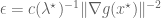
The set U is non-measurable. The set A is measurable.
We will think of our sets as rocks. As explained later, a rock is not “measurable” if its boundary is too jagged. In the above image, the rock 

For 
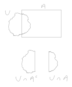
An outer measure uses shrink wrap to approximate the boundary. If A cuts the rock U cleanly then the same “errors” are made when approximating the boundaries of the three objects in the picture, hence Caratheodory’s criterion holds.
The two ingredients of our explanation are that the boundary of
In the above image, the red curve represents the shrink wrap. The outer measure 
When we take 

Consider shrink wrapping
- If the cut made by
- For all other parts of the boundaries of
It follows that
Regardless of whether
From the Beginning
First, it should be appreciated that Caratheodory’s criterion is not magical: it cannot always produce the exact sigma-algebra that you are thinking of, so it suffices to understand why, in certain situations, it is sensible. In particular, this means we can assume that the outer measure we are given, works by considering approximations of a given set
In physical terms, think of measuring the volume of rocks. An outer measure works by wrapping shrink wrap as tightly as possible around the rock, then asking for the volume encased by the shrink wrap. The key point is that if the boundary of the rock is piecewise smooth then the shrink wrap computes its exact volume, whereas if the boundary is sufficiently jagged then the shrink wrap cannot follow the contours perfectly and the shrink wrap (i.e., the outer measure) will exaggerate the true volume of the rock.
It is easy to spot rocks with bad boundaries if the volume of the whole space is finite: look at both the rock and its complement. Place shrink wrap over both of them. If the shrink wrap can follow the contours then it will measure the volume of the two interlocking parts perfectly and the sum of the volumes will equal the volume of the whole space. If not, we know the rock is too ill-shaped to be considered measurable.
If the total volume is infinite then we must zoom in on smaller portions of the boundary. For example, we might take an open ball 


Remarks
- Of course, intuition must be backed up by rigorous mathematics, and it turns out that Caratheodory’s criterion is useful because it is easy to work with and produces the desired sigma-algebra in many situations of interest.
- Our intuitive argument has focused on the boundary of sets. If we consider a Borel measure (one generated by the open sets of a topological space) then we know that open sets are measurable and hence it is indeed the behaviour at the boundary that matters. That said, intuition need not be perfect to be useful.
An Alternative (and Very Simple) Derivation of the Boltzmann Distribution
This note gives a very simple derivation of the Boltzmann distribution that avoids any mention of temperature or entropy. Indeed, the Boltzmann distribution can be understood as the unique distribution with the property that when a large (or even a small!) number of Boltzmann distributions are added together, all the different ways of achieving the same “energy” have the same probability of occurrence, as now explained.
For the sake of a mental image, consider a small volume of gas. This small volume can take on three distinct energy levels, say, 0, 1 and 2. Assume the choice of energy level is random, with corresponding probabilities 

Mathematically, let 


For a fixed 


Since the ordering does not change the probabilities, the problem reduces to the following. Let 


A brute-force computation is informative: write 


Up to a normalising constant, the solutions to 


More generally, we can show that the Boltzmann distribution is the unique distribution with the property that different configurations (or “microstates”) having the same 


Some Comments on the Situation of a Random Variable being Measurable with respect to the Sigma-Algebra Generated by Another Random Variable
If 


First some background. It is a standard result that 


A “direct” proof would endeavour to construct 


Technically, we need a way of extending the definition of
Constructing an appropriate extension requires knowing more about
Consider first the case when 


How did the above construction avoid the problem of the range of 
Consider next the case when 


The above depends crucially on having only finitely many indicator functions. A frequently used principle is that an arbitrary measurable function can be approximated by a sequence of bounded functions with each function being a sum of a finite number of indicator functions (i.e., a simple function). Therefore, the general case can be handled by using a sequence 


Finally, it is remarked that sometimes the monotone class theorem is used in the proof. Essentially, the idea is exactly the same: approximate 


Poles, ROCs and Z-Transforms
Why should all the poles be inside the unit circle for a discrete-time digital system to be stable? And why must we care about regions of convergence (ROC)? With only a small investment in time, it is possible to gain a very clear understanding of exactly what is going on — it is not complicated if learnt step at a time, and there are not many steps.
Step 1: Formal Laurent Series
Despite the fancy name, Step 1 is straightforward. Digital systems operate on sequences of numbers: a sequence of numbers goes into a system and a sequence of numbers comes out. For example, if ![x[n]](https://s0.wp.com/latex.php?latex=x%5Bn%5D&bg=ffffff&fg=555555&s=0&c=20201002)
![y[n] = x[n] + \frac12 x[n-1]](https://s0.wp.com/latex.php?latex=y%5Bn%5D+%3D+x%5Bn%5D+%2B+%5Cfrac12+x%5Bn-1%5D&bg=ffffff&fg=555555&s=0&c=20201002)
How can a specific input sequence be written down, and how can the output sequence be computed?
The direct approach is to specify each individual ![x[n] = 0](https://s0.wp.com/latex.php?latex=x%5Bn%5D+%3D+0&bg=ffffff&fg=555555&s=0&c=20201002)

![x[0] = 1](https://s0.wp.com/latex.php?latex=x%5B0%5D+%3D+1&bg=ffffff&fg=555555&s=0&c=20201002)
![x[1] = 2](https://s0.wp.com/latex.php?latex=x%5B1%5D+%3D+2&bg=ffffff&fg=555555&s=0&c=20201002)
![x[2] = 3](https://s0.wp.com/latex.php?latex=x%5B2%5D+%3D+3&bg=ffffff&fg=555555&s=0&c=20201002)

![y[0] = x[0] + \frac12 x[-1] = 1 + \frac12 \cdot 0 = 1](https://s0.wp.com/latex.php?latex=y%5B0%5D+%3D+x%5B0%5D+%2B+%5Cfrac12+x%5B-1%5D+%3D+1+%2B+%5Cfrac12+%5Ccdot+0+%3D+1&bg=ffffff&fg=555555&s=0&c=20201002)
![y[1] = x[1] + \frac12 x[0] = 2 + \frac12 \cdot 1 = 2\frac12](https://s0.wp.com/latex.php?latex=y%5B1%5D+%3D+x%5B1%5D+%2B+%5Cfrac12+x%5B0%5D+%3D+2+%2B+%5Cfrac12+%5Ccdot+1+%3D+2%5Cfrac12&bg=ffffff&fg=555555&s=0&c=20201002)
The system
Any LTI system has the property that the output is the convolution of the input with the impulse response. For example, the impulse response of 
![y[0] = 1](https://s0.wp.com/latex.php?latex=y%5B0%5D+%3D+1&bg=ffffff&fg=555555&s=0&c=20201002)
![y[1] = \frac12](https://s0.wp.com/latex.php?latex=y%5B1%5D+%3D+%5Cfrac12&bg=ffffff&fg=555555&s=0&c=20201002)
![y[n] = 0](https://s0.wp.com/latex.php?latex=y%5Bn%5D+%3D+0&bg=ffffff&fg=555555&s=0&c=20201002)

![h[0] = 1](https://s0.wp.com/latex.php?latex=h%5B0%5D+%3D+1&bg=ffffff&fg=555555&s=0&c=20201002)
![h[1] = \frac12](https://s0.wp.com/latex.php?latex=h%5B1%5D+%3D+%5Cfrac12&bg=ffffff&fg=555555&s=0&c=20201002)
![h[n] = 0](https://s0.wp.com/latex.php?latex=h%5Bn%5D+%3D+0&bg=ffffff&fg=555555&s=0&c=20201002)
By the definition of convolution, the convolution of a sequence ![h[n]](https://s0.wp.com/latex.php?latex=h%5Bn%5D&bg=ffffff&fg=555555&s=0&c=20201002)
![c[n] = \sum_{m=-\infty}^{\infty} h[m] x[n-m]](https://s0.wp.com/latex.php?latex=c%5Bn%5D+%3D+%5Csum_%7Bm%3D-%5Cinfty%7D%5E%7B%5Cinfty%7D+h%5Bm%5D+x%5Bn-m%5D&bg=ffffff&fg=555555&s=0&c=20201002)
![c[n] = x[n] + \frac12 x[n-1]](https://s0.wp.com/latex.php?latex=c%5Bn%5D+%3D+x%5Bn%5D+%2B+%5Cfrac12+x%5Bn-1%5D&bg=ffffff&fg=555555&s=0&c=20201002)
![y[n]](https://s0.wp.com/latex.php?latex=y%5Bn%5D&bg=ffffff&fg=555555&s=0&c=20201002)
Let’s be honest: writing 

Precisely, the sequence 
![\sum_{n=-\infty}^{\infty} h[n] t^n](https://s0.wp.com/latex.php?latex=%5Csum_%7Bn%3D-%5Cinfty%7D%5E%7B%5Cinfty%7D+h%5Bn%5D+t%5En&bg=ffffff&fg=555555&s=0&c=20201002)


Being able to associate letters with encoded sequences is convenient, hence people will write 
![x[-5] = 2](https://s0.wp.com/latex.php?latex=x%5B-5%5D+%3D+2&bg=ffffff&fg=555555&s=0&c=20201002)
![x[0] = 3](https://s0.wp.com/latex.php?latex=x%5B0%5D+%3D+3&bg=ffffff&fg=555555&s=0&c=20201002)
![x[7] = 1](https://s0.wp.com/latex.php?latex=x%5B7%5D+%3D+1&bg=ffffff&fg=555555&s=0&c=20201002)


Now, there is an added benefit! If the input to our system is 


![y[0]=1, y[1]=2\frac12, y[2] = 4](https://s0.wp.com/latex.php?latex=y%5B0%5D%3D1%2C+y%5B1%5D%3D2%5Cfrac12%2C+y%5B2%5D+%3D+4&bg=ffffff&fg=555555&s=0&c=20201002)
- A formal Laurent series provides a convenient encoding of a discrete-time sequence.
- Convolution of sequences corresponds to multiplication of formal Laurent series.
- Do not think of formal Laurent series as functions of a variable. (They are elements of a commutative ring.) Just treat the variable as a placeholder.
- In particular, there is no need (and it makes no sense) to talk about ROC (regions of convergence) if we restrict ourselves to formal Laurent series.
Step 2: Analytic Functions
This is where the fun begins. We were told not to treat a formal Laurent series as a function, but it is very tempting to do so… so let’s do just that! 🙂 The price we pay though is that we do need to start worrying about ROC (regions of convergence) for otherwise we could end up with incorrect answers.
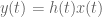
To motivate further our desire to break the rules, consider the LTI system ![y[n] = \frac12 y[n-1] + x[n]](https://s0.wp.com/latex.php?latex=y%5Bn%5D+%3D+%5Cfrac12+y%5Bn-1%5D+%2B+x%5Bn%5D&bg=ffffff&fg=555555&s=0&c=20201002)
![y[n-1]](https://s0.wp.com/latex.php?latex=y%5Bn-1%5D&bg=ffffff&fg=555555&s=0&c=20201002)
![x[0]](https://s0.wp.com/latex.php?latex=x%5B0%5D&bg=ffffff&fg=555555&s=0&c=20201002)
![h[2] = \frac14](https://s0.wp.com/latex.php?latex=h%5B2%5D+%3D+%5Cfrac14&bg=ffffff&fg=555555&s=0&c=20201002)
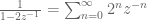
![h[n] = \frac1{2^n}](https://s0.wp.com/latex.php?latex=h%5Bn%5D+%3D+%5Cfrac1%7B2%5En%7D&bg=ffffff&fg=555555&s=0&c=20201002)


There is a more “efficient” representation of 


We know we can encode a sequence using a formal Laurent series, and we can reverse this operation to recover the sequence from the formal Laurent series. In Step 2 then, we just have to consider when we can encode a formal Laurent series as some type (what type?) of function, meaning in particular that it is possible to determine uniquely the formal Laurent series given the function.
Power series (and Laurent series) are studied in complex analysis: recall that every power series has a (possibly zero) radius of convergence, and within that radius of convergence, a power series can be evaluated. Furthermore, within the radius of convergence, a power series (with real or complex coefficients) defines a complex analytic function. The basic idea is that a formal Laurent series might (depending on how quickly the coefficients die out to zero) represent an analytic function on a part of the complex plane.
If the formal Laurent series only contains non-negative powers of 


If the formal Laurent series only contains non-positive powers, that is, 


In the general case, a formal Laurent series decomposes as 
The encoding of a sequence as an analytic function is therefore straightforward in principle: given a formal Laurent series 

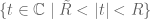
If 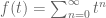


The region 


Readers remembering their complex analysis will not find this bizarre because a holomorphic (i.e., complex differentiable) function generally requires more than one power series to represent it. A power series about a point is only valid up until a pole is encountered, after which another point must be chosen and a power series around that point used to continue the description of the function. When we change points, the coefficients of the power series will generally change. In the above example, the first series 


While it might seem that introducing analytic functions is an unnecessary complication, it actually makes certain calculations simpler! Such a phenomenon happened in Step 1: we discovered convolution of sequences became multiplication of Laurent series (and usually multiplication is more convenient than convolution). In Step 3 we will see how the impulse response of
Step 3: The Z-transform
Define ![y(t) = \sum_{n=-\infty}^\infty y[n] t^n](https://s0.wp.com/latex.php?latex=y%28t%29+%3D+%5Csum_%7Bn%3D-%5Cinfty%7D%5E%5Cinfty+y%5Bn%5D+t%5En&bg=ffffff&fg=555555&s=0&c=20201002)
![x(t) = \sum_{n=-\infty}^\infty x[n] t^n](https://s0.wp.com/latex.php?latex=x%28t%29+%3D+%5Csum_%7Bn%3D-%5Cinfty%7D%5E%5Cinfty+x%5Bn%5D+t%5En&bg=ffffff&fg=555555&s=0&c=20201002)

Note that ![\{\cdots,x[-2],x[-1],x[0],x[1],x[2],\cdots\}](https://s0.wp.com/latex.php?latex=%5C%7B%5Ccdots%2Cx%5B-2%5D%2Cx%5B-1%5D%2Cx%5B0%5D%2Cx%5B1%5D%2Cx%5B2%5D%2C%5Ccdots%5C%7D&bg=ffffff&fg=555555&s=0&c=20201002)
![\{\cdots,y[-2],y[-1],y[0],y[1],y[2],\cdots\}](https://s0.wp.com/latex.php?latex=%5C%7B%5Ccdots%2Cy%5B-2%5D%2Cy%5B-1%5D%2Cy%5B0%5D%2Cy%5B1%5D%2Cy%5B2%5D%2C%5Ccdots%5C%7D&bg=ffffff&fg=555555&s=0&c=20201002)
Intuitively, think of a table (my lack of WordPress skills prevents me from illustrating this nicely). The top row looks like ![\cdots \mid y[-1] \mid y[0] \mid y[1] \mid \cdots](https://s0.wp.com/latex.php?latex=%5Ccdots+%5Cmid+y%5B-1%5D+%5Cmid+y%5B0%5D+%5Cmid+y%5B1%5D+%5Cmid+%5Ccdots&bg=ffffff&fg=555555&s=0&c=20201002)
![\cdots \mid \frac12 y[-2] \mid \frac12 y[-1] \mid \frac12 y[0] \mid \cdots](https://s0.wp.com/latex.php?latex=%5Ccdots+%5Cmid+%5Cfrac12+y%5B-2%5D+%5Cmid+%5Cfrac12+y%5B-1%5D+%5Cmid+%5Cfrac12+y%5B0%5D+%5Cmid+%5Ccdots&bg=ffffff&fg=555555&s=0&c=20201002)
![\cdots \mid x[-1] \mid x[0] \mid x[1] \mid \cdots](https://s0.wp.com/latex.php?latex=%5Ccdots+%5Cmid+x%5B-1%5D+%5Cmid+x%5B0%5D+%5Cmid+x%5B1%5D+%5Cmid+%5Ccdots&bg=ffffff&fg=555555&s=0&c=20201002)
Rigorously, what has just happened is that we are treating a sequence as a vector in an infinite-dimensional vector space: just like ![( y[-1], y[0], y[1] )](https://s0.wp.com/latex.php?latex=%28+y%5B-1%5D%2C+y%5B0%5D%2C+y%5B1%5D+%29&bg=ffffff&fg=555555&s=0&c=20201002)

![( \cdots, y[-1], y[0], y[1], \cdots )](https://s0.wp.com/latex.php?latex=%28+%5Ccdots%2C+y%5B-1%5D%2C+y%5B0%5D%2C+y%5B1%5D%2C+%5Ccdots+%29&bg=ffffff&fg=555555&s=0&c=20201002)

To be able to write the table compactly in vector form, we need some way of going from the vector ![( \cdots, y[-2], y[-1], y[0], \cdots )](https://s0.wp.com/latex.php?latex=%28+%5Ccdots%2C+y%5B-2%5D%2C+y%5B-1%5D%2C+y%5B0%5D%2C+%5Ccdots+%29&bg=ffffff&fg=555555&s=0&c=20201002)

![S(\ ( \cdots, y[-1], y[0], y[1], \cdots ) \ ) = ( \cdots, y[-2], y[-1], y[0], \cdots )](https://s0.wp.com/latex.php?latex=S%28%5C+%28+%5Ccdots%2C+y%5B-1%5D%2C+y%5B0%5D%2C+y%5B1%5D%2C+%5Ccdots+%29%C2%A0%5C+%29+%3D%C2%A0%28+%5Ccdots%2C+y%5B-2%5D%2C+y%5B-1%5D%2C+y%5B0%5D%2C+%5Ccdots+%29&bg=ffffff&fg=555555&s=0&c=20201002)
Letting 

![( \cdots, x[-1], x[0], x[1], \cdots )](https://s0.wp.com/latex.php?latex=%28+%5Ccdots%2C+x%5B-1%5D%2C+x%5B0%5D%2C+x%5B1%5D%2C+%5Ccdots+%29&bg=ffffff&fg=555555&s=0&c=20201002)

Our natural instinct is to collect like terms: if 

While in some cases the expression 

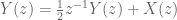
Precisely, since ![\mathbf{y} = ( \cdots, y[-1], y[0], y[1], \cdots )](https://s0.wp.com/latex.php?latex=%5Cmathbf%7By%7D+%3D+%28+%5Ccdots%2C+y%5B-1%5D%2C+y%5B0%5D%2C+y%5B1%5D%2C+%5Ccdots+%29&bg=ffffff&fg=555555&s=0&c=20201002)
![\frac12 t\,y(t) = \frac12 t \sum_{n=-\infty}^\infty y[n] t^n = \sum_{n=-\infty}^\infty \frac12 y[n-1] t^n](https://s0.wp.com/latex.php?latex=%5Cfrac12+t%5C%2Cy%28t%29+%3D+%5Cfrac12+t+%5Csum_%7Bn%3D-%5Cinfty%7D%5E%5Cinfty+y%5Bn%5D+t%5En+%3D+%5Csum_%7Bn%3D-%5Cinfty%7D%5E%5Cinfty+%5Cfrac12+y%5Bn-1%5D+t%5En&bg=ffffff&fg=555555&s=0&c=20201002)
Now, from Step 2, we know that we can think of 

Remark: Actually, the only way to justify rigorously that the above manipulation is valid is to check the answer we have found really is the correct answer. Indeed, to be allowed to perform the manipulations we must assume the existence of a domain on which both 

The remark above shows it is (straightforward but) tedious to verify rigorously that we are allowed to perform the manipulations we want. It is much simpler to go the other way and define a system directly in terms of 
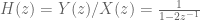
All that remains is to introduce the Z-transform and explain why engineers treat
The Z-transform is simply doing the same as what we have been doing, but using 
The rule that engineers are taught is that when you “take the Z-transform” of 


Step 4: Poles and Zeros
A straightforward but nonetheless rich class of LTI systems can be written in the form ![y[n] = a_1 y[n-1] + a_2 y[n-2] + \cdots + a_p y[n-p] + b_0 x[n] + b_1 x[n-1] + \cdots + b_q x[n-q]](https://s0.wp.com/latex.php?latex=y%5Bn%5D+%3D+a_1+y%5Bn-1%5D+%2B+a_2+y%5Bn-2%5D+%2B+%5Ccdots+%2B+a_p+y%5Bn-p%5D+%2B+b_0+x%5Bn%5D+%2B+b_1+x%5Bn-1%5D+%2B+%5Ccdots+%2B+b_q+x%5Bn-q%5D&bg=ffffff&fg=555555&s=0&c=20201002)

Applying the Z-transform to such a system shows that the impulse response in the Z-domain is a rational function. Note that the product of two rational functions is again a rational function, demonstrating that this class of systems is closed under composition, as stated above. Most of the time, it suffices to work with rational impulse responses.
If 


Poles are important because poles are what determine the regions of convergence and hence they determine when our manipulations in Step 3 are valid. This manifests itself in poles having a physical meaning: as we will see, the closer a pole gets to the unit circle, the less stable a system becomes.
Real-world systems are causal: the output cannot depend on future input. The impulse response 


Let’s look at an unstable system: ![y[n] = 2 y[n-1] + x[n]](https://s0.wp.com/latex.php?latex=y%5Bn%5D+%3D+2+y%5Bn-1%5D+%2B+x%5Bn%5D&bg=ffffff&fg=555555&s=0&c=20201002)

![x[0]=1](https://s0.wp.com/latex.php?latex=x%5B0%5D%3D1&bg=ffffff&fg=555555&s=0&c=20201002)
![y[n] = 2^n](https://s0.wp.com/latex.php?latex=y%5Bn%5D+%3D+2%5En&bg=ffffff&fg=555555&s=0&c=20201002)


If we put a signal that starts at time zero (i.e., 


If we put a signal that started at time 

![x[n] = 1](https://s0.wp.com/latex.php?latex=x%5Bn%5D+%3D+1&bg=ffffff&fg=555555&s=0&c=20201002)

![x[n]=0](https://s0.wp.com/latex.php?latex=x%5Bn%5D%3D0&bg=ffffff&fg=555555&s=0&c=20201002)

There are many different definitions of a sequence being bounded. Three examples are: 1) there exists an ![|x[n]| < M](https://s0.wp.com/latex.php?latex=%7Cx%5Bn%5D%7C+%3C+M&bg=ffffff&fg=555555&s=0&c=20201002)
![\sum_{n=-\infty}^\infty | x[n] | < \infty](https://s0.wp.com/latex.php?latex=%5Csum_%7Bn%3D-%5Cinfty%7D%5E%5Cinfty+%7C+x%5Bn%5D+%7C+%3C+%5Cinfty&bg=ffffff&fg=555555&s=0&c=20201002)
![\sum_{n=-\infty}^{\infty} | x[n] |^2 < \infty](https://s0.wp.com/latex.php?latex=%5Csum_%7Bn%3D-%5Cinfty%7D%5E%7B%5Cinfty%7D+%7C+x%5Bn%5D+%7C%5E2+%3C+%5Cinfty&bg=ffffff&fg=555555&s=0&c=20201002)

![\sum_{n=-\infty}^\infty x[n] z^{-n}](https://s0.wp.com/latex.php?latex=%5Csum_%7Bn%3D-%5Cinfty%7D%5E%5Cinfty+x%5Bn%5D+z%5E%7B-n%7D&bg=ffffff&fg=555555&s=0&c=20201002)
![\sum_{n=-\infty}^\infty |x[n] z^{-n}| < \infty](https://s0.wp.com/latex.php?latex=%5Csum_%7Bn%3D-%5Cinfty%7D%5E%5Cinfty+%7Cx%5Bn%5D+z%5E%7B-n%7D%7C+%3C+%5Cinfty&bg=ffffff&fg=555555&s=0&c=20201002)
![\sum_{n=-\infty}^\infty |x[n]| < \infty](https://s0.wp.com/latex.php?latex=%5Csum_%7Bn%3D-%5Cinfty%7D%5E%5Cinfty+%7Cx%5Bn%5D%7C+%3C+%5Cinfty&bg=ffffff&fg=555555&s=0&c=20201002)


![x[n] = \frac1{n^2}](https://s0.wp.com/latex.php?latex=x%5Bn%5D+%3D+%5Cfrac1%7Bn%5E2%7D&bg=ffffff&fg=555555&s=0&c=20201002)


A sequence
If the ROC of the transfer function
If all the poles of a causal
Note that it follows from earlier remarks that if 

![h[n] = a^n](https://s0.wp.com/latex.php?latex=h%5Bn%5D+%3D+a%5En&bg=ffffff&fg=555555&s=0&c=20201002)
![|h[n]| = |a^n| = 1](https://s0.wp.com/latex.php?latex=%7Ch%5Bn%5D%7C+%3D+%7Ca%5En%7C+%3D+1&bg=ffffff&fg=555555&s=0&c=20201002)

![h[n] = e^{\jmath \omega n}](https://s0.wp.com/latex.php?latex=h%5Bn%5D+%3D+e%5E%7B%5Cjmath+%5Comega+n%7D&bg=ffffff&fg=555555&s=0&c=20201002)


![h[n] = a^n = r^n e^{\jmath \omega n}](https://s0.wp.com/latex.php?latex=h%5Bn%5D+%3D+a%5En+%3D+r%5En+e%5E%7B%5Cjmath+%5Comega+n%7D&bg=ffffff&fg=555555&s=0&c=20201002)

Epilogue
- Although often engineers can get away with just following recipes, it is safer in the long run and easier to remember the recipes if you have spent a bit more time to learn the underlying rationale for when and why the rules work.
- Linear algebra and complex analysis are considered core subjects of an undergraduate mathematics degree because they have such broad applicability: here we saw them play integral roles in discrete-time signal processing.
- This is because the “mathematical behaviour” of Laurent series matches the “physical behaviour” of discrete-time linear time-invariant systems.
- There is a close relationship between the Z-transform and the Fourier transform: just make the substitution
. This is only allowed if the ROC contains the unit circle. The concept of a pole does not explicitly appear in the Fourier domain because, rather than permit
- When it comes to system design, understanding where the poles and zeros are can be more productive than trying to understand the whole frequency spectrum.
